Neural Network from Scratch in Python
In this post we will implement a 2-layer neural network from scratch using Python and numpy. We won’t derive the mathematics but I will try to give you an intuition of what we are trying to accomplish.
Generating a Dataset
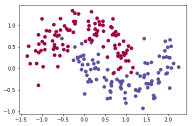
Let’s start by creating a dataset that we can use to train our neural network. We will make use of scikit-learn to create the dataset.
1
2
3
4
# import the necessary packages
import numpy as np
from sklearn import datasets
import matplotlib.pyplot as plt
1
2
3
4
5
%matplotlib inline
# Generate a dataset and plot it
np.random.seed(0)
X, y = datasets.make_moons(200, noise=0.20)
plt.scatter(X[:,0], X[:,1], s=40, c=y, cmap=plt.cm.Spectral)

We have 200 training examples and 2 features which will help us in training our neural network.
1
2
3
4
5
# X and Y should be of the shape (no_of_features, no_of_examples)
X = X.T
y = y.reshape(y.shape[0],1).T
print(X.shape)
print(y.shape)
Training a Neural Network.
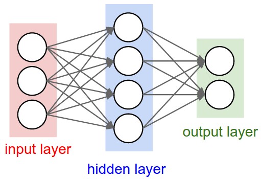
Neural neworks are typically organized in layers. Layers are made up of a number of interconnected ‘nodes’ which contain an ‘activation function’.
Patterns are presented to the network via the ‘input layer’, which communicates to one or more ‘hidden layers’ where the actual processing is done via a system of weighted ‘connections’.
The hidden layers then link to an ‘output layer’ where the answer is output as shown in the figure below.

Define the neural network structure
Let us first start by defining some variables which will determine the number of input features, number of hidden layers and number of output layer.
1
2
3
4
5
m = X.shape[1] #number of examples
n_x = X.shape[0] # input layer
n_h = 1
n_y = y.shape[0] # output layer
learning_rate = 0.1 # learning rate
Initialize the weights and biases.
Weights in a NN are the most important factor in converting an input to impact the output. This is similar to slope in linear regression, where a weight is multiplied to the input to add up to form the output. Weights are numerical parameters which determine how strongly each of the neurons affects the other.
Bias is like the intercept added in a linear equation. It is an additional parameter which is used to adjust the output along with the weighted sum of the inputs to the neuron.
We will initialize weights matrices with random values and bias vectors as zero. To know more about why we initailize weights to random values refer this stackoverflow thread.
1
2
3
4
5
6
7
8
9
10
11
12
def initialize_parameters(n_x, n_h, n_y):
    np.random.seed(2)
    W1 = np.random.randn(n_h, n_x) * 0.01
    b1 = np.zeros((n_h, 1))
    W2 = np.random.randn(n_y, n_h) * 0.01
    b2 = np.zeros((n_y,1))

    parameters = {"W1": W1,
                  "b1": b1,
                  "W2": W2,
                  "b2": b2}
    return parameters
Activation function
The activation function transforms the inputs of the layer into its outputs. A nonlinear activation function is what allows us to fit nonlinear hypotheses.
Common choices for activation functions are tanh, the sigmoid function, or ReLUs. More details about these activation functions can be found here.
1
2
def sigmoid(X):
    return 1/(1 + np.exp(-X))
Forward Progagation
The natural step to do after initialising the model at random, is to check its performance. We start from the input we have, we pass them through the network layer and calculate the actual output of the model. The output is calculated using the below equations.
For one example :
1
2
3
4
5
6
7
8
9
10
11
12
13
14
15
16
17
def forward_propagation(X, parameters):

    W1 = parameters["W1"]
    b1 = parameters["b1"]
    W2 = parameters["W2"]
    b2 = parameters["b2"]

    Z1 = np.dot(W1, X) + b1
    A1 = np.tanh(Z1)
    Z2 = np.dot(W2, A1) + b2
    A2 = sigmoid(Z2)

    cache = {"Z1": Z1,
             "A1": A1,
             "Z2": Z2,
             "A2": A2}
    return A2, cache
Loss Function
Loss function is used to measure the inconsistency between predicted value (yhat) and actual label (y). It is a non-negative value, where the robustness of model increases along with the decrease of the value of loss function.
1
2
3
4
5
6
def compute_cost(A2, Y, parameters):
    logprobs = np.multiply(np.log(A2),Y) + np.multiply(np.log(1-A2),(1-Y))
    cost = -(1/m) * np.sum(logprobs)

    cost = np.squeeze(cost)
    return cost
Back propagation
Error is calculated between the expected outputs and the outputs forward propagated from the network. These errors are then propagated backward through the network from the output layer to the hidden layer, updating weights as they go.
We won’t derive the maths behind this as it will involve a fair amount of calculus but an excellent explanation is provided here
1
2
3
4
5
6
7
8
9
10
11
12
13
14
15
16
17
18
19
20
21
def backward_propagation(parameters, cache, X, Y):

  W1 = parameters['W1']
  W2 = parameters['W2']

  A1 = cache['A1']
  A2 = cache['A2']

  dZ2 = A2 - Y
  dW2 = (1/m) * np.dot(dZ2, A1.T)
  db2 = (1/m) * np.sum(dZ2, axis=1, keepdims=True)

  dZ1 = np.dot(W2.T, dZ2) * (1 - A1**2)
  dW1 = (1/m) * np.dot(dZ1, X.T)
  db1 = (1/m) * np.sum(dZ1, axis=1, keepdims=True)

  grads = {"dW1": dW1,
           "db1": db1,
           "dW2": dW2,
           "db2": db2}
  return grads
Optimization with Gradient Descent
Back propagation moves the error information from the end of the network to all the weights inside the network. Optimization algorithms like Gradient Descent will help us in finding the optimum values of weights which will minimize the loss function.
General gradient descent rule: where is the learning rate and represents a parameter.
More detailed explanation about gradient descent can be found here
1
2
3
4
5
6
7
8
9
10
11
12
13
14
15
16
17
18
19
20
21
22
23
def update_parameters(parameters, grads):

    W1 = parameters['W1']
    b1 = parameters['b1']
    W2 = parameters['W2']
    b2 = parameters['b2']

    dW1 = grads['dW1']
    db1 = grads['db1']
    dW2 = grads['dW2']
    db2 = grads['db2']

    W1 = W1 - learning_rate * dW1
    b1 = b1 - learning_rate * db1
    W2 = W2 - learning_rate * dW2
    b2 = b2 - learning_rate * db2

    parameters = {"W1": W1,
                  "b1": b1,
                  "W2": W2,
                  "b2": b2}

    return parameters
Implementation
Now we have all the methods defined which will help us in training a 2-Layer NN. Let us write a method which will call all the methods mentioned above.
1
2
3
4
5
6
7
8
9
10
11
12
13
14
15
16
17
18
19
def nn_model(X, Y, n_h, num_iterations = 10000, print_cost=False):

    parameters = initialize_parameters(n_x, n_h, n_y)
    W1 = parameters['W1']
    b1 = parameters['b1']
    W2 = parameters['W2']
    b2 = parameters['b2']

    for i in range(0, num_iterations):

        A2, cache = forward_propagation(X, parameters)
        cost = compute_cost(A2, Y, parameters)
        grads = backward_propagation(parameters, cache, X, Y)
        parameters = update_parameters(parameters, grads)

        if print_cost and i % 1000 == 0:
            print ("Cost after iteration %i: %f" %(i, cost))

    return parameters
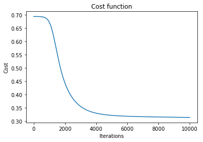
Train the model for 10000 epochs and plot the cost.
1
2
3
4
5
parameters, costs = nn_model(X, y, n_h = 1, num_iterations=10000, print_cost=True)
plt.plot(costs)
plt.xlabel('Iterations')
plt.ylabel('Cost')
plt.title('Cost function')
Cost after iteration 0: 0.693127
Cost after iteration 1000: 0.671018
Cost after iteration 2000: 0.442552
Cost after iteration 3000: 0.354652
Cost after iteration 4000: 0.329080
Cost after iteration 5000: 0.320810
Cost after iteration 6000: 0.317526
Cost after iteration 7000: 0.315824
Cost after iteration 8000: 0.314688
Cost after iteration 9000: 0.313792

I hope this gives you an intuition about neural networks. The entire code is available as a Jupyter notebook here
