Fashion MNIST using ConvNets
Researchers at Zalando, an e-commerce company, introduced Fashion MNIST as a drop-in replacement for the original MNIST dataset. Like MNIST, Fashion MNIST consists of a training set consisting of 60,000 examples belonging to 10 different classes and a test set of 10,000 examples.
Each example is a 28x28 grayscale image (just like the images in the original MNIST), associated with a label from 10 classes (t-shirts, trousers, pullovers, dresses, coats, sandals, shirts, sneakers, bags, and ankle boots).
Let us use TensorFlow to implement a Convolutional Network to classify these images.
Importing the Dataset
Fashion MNIST can be imported in the same way as MNIST data set in Tensorflow. While importing the dataset, let’s apply one-hot encoding to our class variables.
1
2
3
4
5
import tensorflow as tf
import matplotlib.pyplot as plt

from tensorflow.examples.tutorials.mnist import input_data
fashion_mnist = input_data.read_data_sets("data/fashion", one_hot=True)
Please note that the above code assumes that the dataset has been saved in data/fashion directory. It can downloaded from here
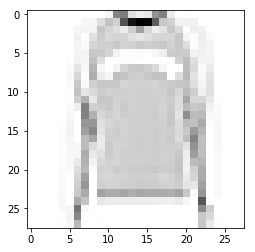
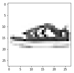
Let’s take a look at some of the examples from the dataset.
1
2
3
4
5
6
7
8
%matplotlib inline
sample_1 = fashion_mnist.train.images[100].reshape(28,28)
plt.imshow(sample_1, cmap='Greys')
plt.show()

sample_2 = fashion_mnist.train.images[500].reshape(28,28)
plt.imshow(sample_2, cmap='Greys')
plt.show()


Network Parameters
Define some hyperparameters that will be used by the network.
1
2
3
4
5
6
7
8
9
10
# Training Parameters
learning_rate = 0.001
num_steps = 500
batch_size = 128
display_step = 10

# Network Parameters
num_input = 784 # Data input (Image shape: 28*28)
num_classes = 10 # Total classes (0-9 labels)
dropout = 0.75 # Dropout probability
Creating Placeholders
A placeholder in TensorFlow is simply a variable that we will assign data to at a later date. It allows us to create our operations and build our computation graph.
1
2
3
4
5
def create_placeholders():
    X = tf.placeholder(tf.float32, [None, num_input])
    Y = tf.placeholder(tf.float32, [None, num_classes])
    keep_prob = tf.placeholder(tf.float32)
    return X, Y, keep_prob
Weights and Biases
We need to initalize Weights and Biases that will be used by our convolutional layer as well as the fully connected layer. These parameters will be updated during the training.
1
2
3
4
5
6
7
8
9
10
11
12
13
14
15
16
17
weights = {
    # 5x5 conv, 1 input, 32 outputs
    'wc1': tf.Variable(tf.random_normal([5, 5, 1, 32])),
    # 5x5 conv, 32 inputs, 64 outputs
    'wc2': tf.Variable(tf.random_normal([5, 5, 32, 64])),
    # fully connected, 7*7*64 inputs, 1024 outputs
    'wf1': tf.Variable(tf.random_normal([7*7*64, 1024])),
    # 1024 inputs, 10 outputs
    'out': tf.Variable(tf.random_normal([1024, num_classes]))
}

biases = {
    'bc1': tf.Variable(tf.random_normal([32])),
    'bc2': tf.Variable(tf.random_normal([64])),
    'bf1': tf.Variable(tf.random_normal([1024])),
    'out': tf.Variable(tf.random_normal([num_classes]))
}
Convolutional Layer
The first layer in a Convolutional Neural Network or ConvNets is always a Convolutional Layer. The primary purpose of Convolution in case of a ConvNet is to extract features from the input image. Convolution preserves the spatial relationship between pixels by learning image features using small squares of input data.
I will not go into the details of Convolutional layer but an excellent explanation is provided here
1
2
3
4
5
def conv2d(x, W, b, strides = 1):
    x = tf.nn.conv2d(x, W, strides=[1, strides, strides, 1],
    		padding='SAME')
    x = tf.nn.bias_add(x, b)
    return tf.nn.relu(x)
Pooling Layer
It is common to periodically insert a Pooling layer in-between successive Conv layers in a ConvNet architecture. Pooling (also called subsampling or downsampling) reduces the dimensionality of each feature map but retains the most important information.
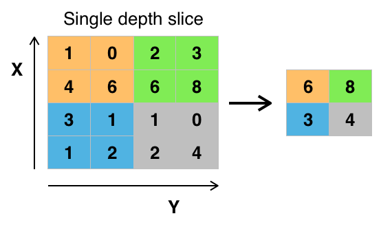
Pooling can be of different types: Max, Average, Sum etc, most popular being Max Pooling, where the maximum pixel value within each chunk is taken.
1
2
3
def maxpool2d(x):
    return tf.nn.max_pool(x, ksize=[1,2,2,1], strides=[1,2,2,1],
    			padding='SAME')
A diagrammatical illustration of 2×2 max-pooling is given below.

Building the Classification Model
Now we will start building our CNN based model. It consists of 2 convolutional layer each followed by max pooling. The output of the second max pooling is flattened and fed into a fully connected layer with 1024 neurons with ReLU activation. This is then given to a 10 neurons Softmax activation function.
1
2
3
4
5
6
7
8
9
10
11
12
13
14
15
16
17
18
19
20
21
22
23
24
25
26
27
28
29
def conv_net(x, weights, biases, dropout):

    # Fashion MNIST data is 1D input vector with 784 features(28*28).
    #Reshape it to a 4D tensor  with the second and third dimensions
    #corresponding to image width and height,
    #and the final dimension corresponding to the number of color channels.
    x = tf.reshape(x, [-1, 28, 28, 1])

    # Convolution layer
    conv1 = conv2d(x, weights['wc1'], biases['bc1'])
    #Max pooling
    conv1 = maxpool2d(conv1)

    #Convolution layer
    conv2 = conv2d(conv1, weights['wc2'], biases['bc2'])
    #Max pooling
    conv2 = maxpool2d(conv2)

    #Fully connected layer
    fc1 = tf.reshape(conv2, [-1, 7*7*64])
    fc1 = tf.add(tf.matmul(fc1, weights['wf1']), biases['bf1'])
    fc1 = tf.nn.relu(fc1)

    #Apply dropout
    fc1 = tf.nn.dropout(fc1, dropout)

    #Output
    output = tf.matmul(fc1, weights['out']) + biases['out']
    return output
Computing Cost
First let us get the predicted values and then try to determine the cost between the target predicted by convnet and the actual target class.
1
2
3
4
5
6
7
8
9
10
11
X, Y, keep_prob = create_placeholders()

#Forward Propagation
logits = conv_net(X, weights, biases, keep_prob)
prediction = tf.nn.softmax(logits)

#Define the cost function and back propagate using Adam Optimizer
#which minimizes the loss
loss = tf.reduce_mean(tf.nn.softmax_cross_entropy_with_logits
            (logits=logits, labels=Y))
train = tf.train.AdamOptimizer(learning_rate=learning_rate).minimize(loss)
Training and Evaluation
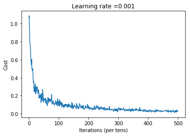
I have trained the model for 500 epochs, printing the cost after every 100 epochs. This gives an accuracy of 81.92% on test set images
1
2
3
4
5
6
7
8
9
10
11
12
13
14
15
16
17
18
19
20
21
22
23
24
25
26
27
init = tf.global_variables_initializer()
costs = []
with tf.Session() as sess:

    sess.run(init)
    for step in range(num_steps):
        minibatch_cost = 0
        batch_x, batch_y = fashion_mnist.train.next_batch(batch_size)
        #Run the session
        _, temp_cost = sess.run([train, loss],
                feed_dict = {X:batch_x, Y:batch_y, keep_prob:dropout})
        minibatch_cost += temp_cost / fashion_mnist.train.num_examples

        if step % 100 == 0:
            print ("Cost after epoch %i: %f" % (step, minibatch_cost))
        if step % 1 == 0:
            costs.append(minibatch_cost)

    # Evaluate model
    correct_pred = tf.equal(tf.argmax(prediction, 1), tf.argmax(Y, 1))
    accuracy = tf.reduce_mean(tf.cast(correct_pred, tf.float32))

    #Calculate accuracy of Fashion MNIST Test images
    print('Testing Accuracy:', sess.run(accuracy,
                        feed_dict={X: fashion_mnist.test.images,
                        Y: fashion_mnist.test.labels,
                        keep_prob: 1.0}))
Cost after epoch 0: 1.659150
Cost after epoch 100: 0.128432
Cost after epoch 200: 0.115758
Cost after epoch 300: 0.051636
Cost after epoch 400: 0.035131
Testing Accuracy: 0.8192
Plot the cost function
1
2
3
4
5
6
7
#Plot the cost function
import numpy as np
plt.plot(np.squeeze(costs))
plt.ylabel('Cost')
plt.xlabel('Iterations (per tens)')
plt.title("Learning rate =" + str(learning_rate))
plt.show()

The entire code is available on github
